Finding Collisions in MD4
Sep 10, 2017On and off for the past couple of years, my friend Ray and I have been working through the Cryptopals Crypto Challenges, a series of exercises split across eight sets that explore modern cryptographic protocols and their weaknesses. The challenges start out pretty easy, but as you move forward, the attacks you’re asked to implement become increasingly difficult.
This post is about challenge 55, “MD4 Collisions.” In it, you’re asked to implement Wang’s 2004 attack on the MD4 hash function. The attack itself is pretty difficult: as far as Ray and I can tell, no one has posted a solution to it online. (There is this code from Bishop Fox, but it consists solely of a dense, 500-line, uncommented C program).
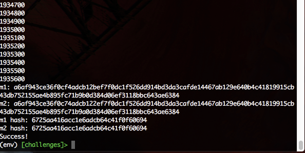
After several days of work, our script finally spit out a brand new collision:
In this post we’ll talk about the attack and our implementation in detail.
How MD4 works
MD4 was invented by Ron Rivest in 1990, back when no one really knew how to design cryptographically-secure hash functions. It uses a 128-bit message digest, meaning that its internal state and the hash that it outputs is 128 bits, or 16 bytes. Internally, MD4 treats this state as four 32-bit integers, which we’ll call \( a \), \( b \), \( c \), and \( d \). These are initialized to four fixed constants at the start of hash function.
MD4 uses a Merkle–Damgård construction, which means that the message that we want to hash is first padded to a multiple of a specific block size (16 bytes for MD4). Then, the hash function reads in the message one block at at time and uses the contents of the block to scramble its internal state. The final internal state after reading all the blocks of the message becomes the actual hash.
Several hash functions (including SHA-256) use Merkle-Damgård constructions, so the main thing that differentiates them is how they modify their state for a given message block. MD4’s modification consists of 48 operations split up into 3 rounds. Each of these operations look something like this:
\[ a = ((a + f(b, c, d) + m[i]) \mod 2^{32}) \lll s \]
where \(f\) is some non-linear function that is unique to each of the three rounds and \(m[i]\) represents the \(i\)th little-endian 32-bit word of our message block. Each operation updates one of the state variables and the updates cycle between the variables in a regular order (\(a\) then \(d\) then \(c\) then \(b\)). Each round consists of 16 of these operations, each of which mix in a different \(m[i]\) resulting in four updates to each of the state variables per round.
You can stare at the full code below to get a better sense of how it all works:
def _f(x, y, z): return x & y | ~x & z
def _g(x, y, z): return x & y | x & z | y & z
def _h(x, y, z): return x ^ y ^ z

def _f1(a, b, c, d, k, s, X): return _left_rotate(a + _f(b, c, d) + X[k], s)
def _f2(a, b, c, d, k, s, X): return _left_rotate(a + _g(b, c, d) + X[k] + 0x5a827999, s)
def _f3(a, b, c, d, k, s, X): return _left_rotate(a + _h(b, c, d) + X[k] + 0x6ed9eba1, s)


def md4_compress(block, state=None):

  if not state: state = [0x67452301, 0xefcdab89, 0x98badcfe, 0x10325476]
  a, b, c, d = h0, h1, h2, h3 = state

  x = list(little_endian_words(block))

  a = _f1(a,b,c,d, 0, 3, x)
  d = _f1(d,a,b,c, 1, 7, x)
  c = _f1(c,d,a,b, 2,11, x)
  b = _f1(b,c,d,a, 3,19, x)
  a = _f1(a,b,c,d, 4, 3, x)
  d = _f1(d,a,b,c, 5, 7, x)
  c = _f1(c,d,a,b, 6,11, x)
  b = _f1(b,c,d,a, 7,19, x)
  a = _f1(a,b,c,d, 8, 3, x)
  d = _f1(d,a,b,c, 9, 7, x)
  c = _f1(c,d,a,b,10,11, x)
  b = _f1(b,c,d,a,11,19, x)
  a = _f1(a,b,c,d,12, 3, x)
  d = _f1(d,a,b,c,13, 7, x)
  c = _f1(c,d,a,b,14,11, x)
  b = _f1(b,c,d,a,15,19, x)

  a = _f2(a,b,c,d, 0, 3, x)
  d = _f2(d,a,b,c, 4, 5, x)
  c = _f2(c,d,a,b, 8, 9, x)
  b = _f2(b,c,d,a,12,13, x)
  a = _f2(a,b,c,d, 1, 3, x)
  d = _f2(d,a,b,c, 5, 5, x)
  c = _f2(c,d,a,b, 9, 9, x)
  b = _f2(b,c,d,a,13,13, x)
  a = _f2(a,b,c,d, 2, 3, x)
  d = _f2(d,a,b,c, 6, 5, x)
  c = _f2(c,d,a,b,10, 9, x)
  b = _f2(b,c,d,a,14,13, x)
  a = _f2(a,b,c,d, 3, 3, x)
  d = _f2(d,a,b,c, 7, 5, x)
  c = _f2(c,d,a,b,11, 9, x)
  b = _f2(b,c,d,a,15,13, x)

  a = _f3(a,b,c,d, 0, 3, x)
  d = _f3(d,a,b,c, 8, 9, x)
  c = _f3(c,d,a,b, 4,11, x)
  b = _f3(b,c,d,a,12,15, x)
  a = _f3(a,b,c,d, 2, 3, x)
  d = _f3(d,a,b,c,10, 9, x)
  c = _f3(c,d,a,b, 6,11, x)
  b = _f3(b,c,d,a,14,15, x)
  a = _f3(a,b,c,d, 1, 3, x)
  d = _f3(d,a,b,c, 9, 9, x)
  c = _f3(c,d,a,b, 5,11, x)
  b = _f3(b,c,d,a,13,15, x)
  a = _f3(a,b,c,d, 3, 3, x)
  d = _f3(d,a,b,c,11, 9, x)
  c = _f3(c,d,a,b, 7,11, x)
  b = _f3(b,c,d,a,15,15, x)

  return [(h0 + a) & 0xffffffff, (h1 + b) & 0xffffffff, (h2 + c) & 0xffffffff, (h3 + d) & 0xffffffff]
Wang’s Attack
Since MD4 is a 128-bit hash function, it should require on the order of \( 2^{128} \) computations to produce a preimage, and on the order of \( 2^{64} \) computations to produce a collision (because of the birthday paradox). However, soon after it was published, weaknesses were discovered which rendered attacks much more feasible. Indeed, Wang’s attack claims to be able to find a collision with only \( 2^8 \) computations.
Wang’s attack uses a technique called differential cryptanalysis, the same method which was used to break many block ciphers in the past. (More recently, the hash function Curl which formed the basis of the IOTA blockchain was broken using differential cryptanalysis).
Essentially, differential cryptanalysis involves carefully examining how minor differences in inputs lead to differences in outputs. What Wang found was that for a certain subset of messages that adhered to a number of constraints, a particular differential resulted in a completely identical output (i.e. a hash collision). Wang called these messages “weak.”
For any weak message \(m\), Wang claimed that the message \(m’ \neq m\) resulted in a collision where \(m’\) is defined as:
\[ \Delta m = m’ - m = (\Delta m_0, \Delta m_1, \cdots, \Delta m_{15})\] \[ \Delta m_1 = 2^{31}, \Delta m_2 = 2^{31} - 2^{28}, \Delta m_{12} = - 2^{16} \] \[ \Delta m_i = 0, 0 \le i \le 15, i \neq 1, 2, 12 \]
Here, \(m_i\) is defined as the \(i\)th 32-bit little-endian word of the message \(m\).
So, what makes a message \(m\) weak? In her paper, Wang listed 121 “constraints” that she claimed were sufficient to ensure that a message was weak. (Later research has shown that 2 additional constraints are actually required for sufficiency).
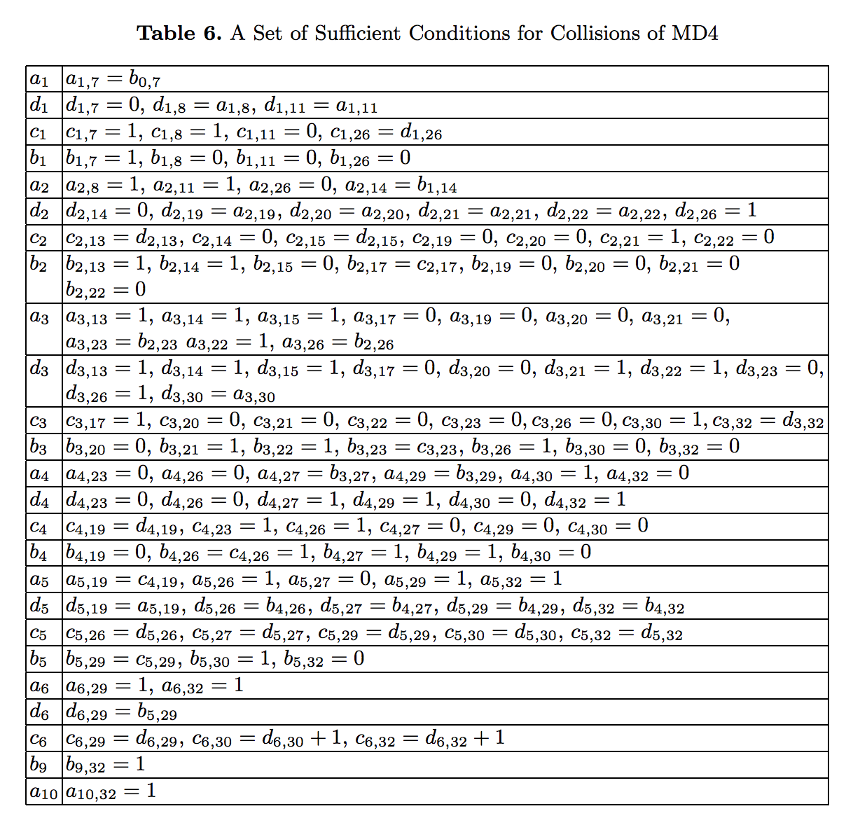
Each of these constraints is a condition on a single bit of a state variable at some point after one of the 48 updates. For example, the first constraint is \(a_{1, 7} = b_{0, 7}\). This means that after \(a\)’s first update, the 7th bit of \(a\) (1-indexing) should equal the 7th bit of \(b\).
The constraints are (more-or-less) independent of each other, so if you have some way of generating random messages that satisfy \(k\) of the 121 constraints, then on average \(2^{121 - k}\) of the messages you generate should satisfy the rest of the constraints (just by chance) and be weak.
It’s relatively easy to satisfy the first few constraints, but as you go on it becomes harder and harder because with each new constraint you have to ensure that you don’t mess up all of the prior ones. In our attack we satisfied all but 19 of Wang’s constraints and 1 out of the 2 additional constraints listed in the improved attack. This suggests that we need to generate \(2^{20}\) or around 1 million messages to find a collision. This seems to be borne out by experimental results.
But wait: how exactly did Wang produce these 100-odd constraints? Her paper doesn’t say much in this regard and other accounts online indicate that they were produced mostly by staring really hard at MD4.
Implementing Wang's MD4 collision attack... and all the papers I've read say that she found the right difference patterns by "intuition" x.x
— Ray Wang (@ghostly_gray) September 8, 2017
We don’t actually need to know how Wang arrived at the right constraints to carry out our attack, but it would be nice to understand this part better. If you have a good explanation, please let me know!
First-round constraints
All constraints that deal with updates to state variables made in the first round are pretty straightforward to enforce. This is because each of the 16 first-round updates involves a different \(m[i]\) which means that we can alter each word of \(m[i]\) independently without wrecking the rest of our constraints.
Enforcing a constraint involves nothing more than adjusting the computed state variable to make the constraint true, and then using algebra to solve for the \(m[i]\) that results in the new state variable. For example, to enforce the constraint \(a_{1, 7} = b_{0, 7}\), we first compute our original \(a_1\):
\[a_1 = ((a_0 + f(b_0, c_0, d_0) + m[0]) \mod 2^{32}) \lll 3 \]
adjust it to meet the constraint:
\[a_1’ = a_1 \oplus ((a_1 \oplus b_0) \wedge (1 \ll i)) \]
and then compute a new \(m[0]’\) that results in this \(a_1’\):
\[ m[0]’ = (a_1’ \ggg 3) - a_0 - f(b_0, c_0, d_0) \mod 2^{32}. \]
Several updates have multiple constraints on different bits that need to be enforced. For these, simply compute the new state variable that satisfies all the constraints, and follow the process above to derive the corresponding \(m[i]\).
There are really only 3 different types of constraints, so its helpful to write some helper functions to do most of the heavy lifting:
# helper methods to adjust the state variables
# to satisfy Wang's constraints
def correct_bit_equal(u, v, i):
  b = u
  u ^= ((u ^ v) & (1 << i))
  # print('EQU {} --> {} ({})'.format(b, u, 'Changed' if b != u else 'Same'))
  return u

def correct_bit_zero(u, i):
  b = u
  u &= ~(1 << i)
  # print('ZER {} --> {} ({})'.format(b, u, 'Changed' if b != u else 'Same'))
  return u

def correct_bit_one(u, i):
  b = u
  u |= (1 << i)
  # print('ONE {} --> {} ({})'.format(b, u, 'Changed' if b != u else 'Same'))
  return u

# enforce first-round constraints
def do_op(state, j, i, s, x, constraints):
  # perform the MD4 operation
  v = lrot(state[j%4] +
          f(state[(j+1)%4], state[(j+2)%4], state[(j+3)%4]) +
          x[i], s)

  # correct the bits according to the constraints
  for constraint in constraints:
    if   constraint[0] == 'equ':
      v = correct_bit_equal(v, state[(j+1)%4], constraint[1])
    elif constraint[0] == 'zer':
      v = correct_bit_zero(v, constraint[1])
    elif constraint[0] == 'one':
      v = correct_bit_one(v, constraint[1])

  # compute the correct message word using algebra
  x[i] = rrot(v, s) - state[j%4] - f(state[(j+1)%4], state[(j+2)%4], state[(j+3)%4])
  x[i] = x[i] % (1 << 32)

  # update the state
  state[j%4] = v
  return
Then, you can just write down your constraints in an array and have your code run through and enforce all of them.
Second-round constraints
With just first-round constraints, any randomly generated message can be adjusted to be weak with probability about \(2^{-26}\). This is still too big to make generating collisions super convenient, so we should enforce some second-round constraints to speed up our script.
The first second-round constraint is \(a_{5, 19} = c_{4,19}\). If we just enforce it as we did above we might encounter a problem: in the process of enforcing it we’ll have to recompute a value for \(m[0]\), however this new value might mess up our constraints from the very first operation which also involved \(m[0]\).
It turns out this isn’t actually true (at least for the first few second-round constraints). Because the bits involved in the constraints for the 17th update do not overlap at all with the bits involved in the constraints for the 1st update, they also involve entirely separate bits of \(m[0]\), so we’re safe.
However, there is another, more subtle problem. When we change \(m[0]\), we’re also retroactively changing the value of \(a_1\), which was involved in the calculations for the 2nd, 3rd, 4th, and 5th operations. This will ruin the rest of our constraints.
Wang’s solution to this involves “multi-step corrections.” The principle is essentially “it’s ok if \(a_1\) changes, but don’t let the changes propagate any further than that”. For each of the four operations that \(a_1\) was involved with, adjust the corresponding \(m[i]\) such that the updated state variable remains the same when the operation is performed with the new value of \(a_1\).
Here’s what that looks like in terms of math:
This is the 17th update involving \(a_5\):
\[a_5 = ((a_4 + g(b_4, c_4, d_4) + m[0] + \text{0x5a827999}) \mod 2^{32}) \lll 3 \]
Suppose we’ve computed our adjusted \(a_5’\) to meet our 17th update constraints. Then we recompute \(m[0]\) as:
\[m[0]’ = (a_5’ \ggg 3) - a_4 - g(b_4, c_4, d_4) - \text{0x5a827999} \mod 2^{32} \]
This retroactively changes the value of \(a_1\) to:
\[a_1’ = ((a_0 + f(b_0, c_0, d_0) + m[0]’) \mod 2^{32}) \lll 3 \]
from the first update. Now, the second update looks like:
\[d_1 = ((d_0 + f(a_1, b_0, c_0) + m[1]) \mod 2^{32}) \lll 7 \]
Using algebra, we can recompute \(m[1]\) such that \(d_1\)’s value won’t change when this update is performed with \(a_1’\) instead of \(a_1\):
\[m[1]’ = (d_1 \ggg 7) - d_0 - f(a_1’,b_0, c_0) \mod 2^{32} \]
And we can do the same thing for \(m[2], m[3], \) and \(m[4]\):
\[m[2]’ = (c_1 \ggg 11) - c_0 - f(d_1, a_1’, b_0) \mod 2^{32} \] \[m[3]’ = (b_1 \ggg 19) - b_0 - f(c_1, d_1, a_1’) \mod 2^{32} \] \[m[4]’ = (a_2 \ggg 3) - a_1’ - f(b_1, c_1, d_1) \mod 2^{32} \]
It’s actually not immediately clear that this actually works. Sure, the only thing that has changed is \(a_1\), but \(a_1\) is involved in three constraints. It’s certainly possible that we could have messed these up. It turns out that since the bits of the constraints that \(a_1\) is involved with are far enough away from the bits that we’re flipping to satisfy \(d_5\), we’re fine.
However, this is no longer true for the next set of second-round updates. Although Wang claims that you can use the same technique to enforce these, in practice I found that I could only reliably enforce the last two of them, involving \(d_{5,29}\) and \(d_{5,32}\), without wrecking my constraints for the fifth update. (Wang also claims, confusingly, that it’s important to enforce second-round constraints in bit-order one at a time, but this is also not true.)
Implementation details
Here are a bunch of other things to consider when actually implementing the attack:
- You’ll probably mess up when you try to enforce the second-round constraints. When you do, it’s helpful to have a constraint-checker that is constantly verifying that all of your constraints are still satisfied before you actually check for a collision. Sprinkle a bunch of asserts to make sure you catch errors early.
- When generating random message blocks to adjust, use python’s
randomlibrary instead ofos.urandom. The latter is cryptographically-secure (and slow) while the former is not, but much faster. - The running time of the code is probably dominated by running MD4 to check that you actually found a collision. It would be nice if this part was super fast, preferably in the form of a python library that calls into C. Sadly, python’s latest version of
hashlibno longer supports MD4 (presumably to stop people from ever using it again), so my MD4 check was pure python. - Speaking of performance, it’s probably better to just write the whole script in a compiled language like C / C++ or Go.
- You could avoid extra MD4 computations by checking the rest of the constraints that you haven’t enforced and halting if you find one of them to not be true.
The collision
On 9/9/17 at 10:29 pm, our script returned its first-ever collision after trying around 2 million random starting messages. This was the collision we generated:
m1 = a6af943ce36f0cf4adcb12bef7f0dc1f526dd914bd3da3cafde14467ab129e640b4c41819915cb43db752155ae4b895fc71b9b0d384d06ef3118bbc643ae6384
m2 = a6af943ce36f0c74adcb122ef7f0dc1f526dd914bd3da3cafde14467ab129e640b4c41819915cb43db752155ae4b895fc71b9a0d384d06ef3118bbc643ae6384
hash = 6725aa416acc1e6adcb64c41f0f60694
Perhaps right now you’re thinking “So what? it’s just a collision. What really matters is a second pre-image”. First of all, this is definitely not true. There are plenty of applications that rely on the collision resistance of its hash functions. There are even cool cryptographic attacks that involve exploiting the difference in difficulty between finding second pre-images and collisions.
But more importantly, cryptographic attacks always get better. Just a year later, researchers presented a viable second-preimage attack on MD4 using a different differential.
The good news is that cryptographers seem to have finally figured out how to get hash functions right. It used to be that every invented hash function would experience a predictable life-to-death cycle, but so far both the SHA-2 and SHA-3 families look pretty good. Then again, who knows? Maybe a decade from now some college student will be solving cryptopals challenge 107: “SHA-256 Collisions.”
You can read our full attack script here.